線形重回帰分析
モデルフィット
データは南風原朝和 (2002). 心理統計学の基礎――統合的理解のために―― 有斐閣から。感謝
		# p226 。表8-1。50組の母子の協調性データ。

		x1 <- c(12, 12, 7, 17, 14, 9, 10, 13, 15, 12, 12, 15, 11, 14, 17, 17, 16, 15, 15, 10, 12, 9, 12, 12, 19, 11, 14, 15, 15, 15, 16, 15, 12, 10, 11, 12, 15, 13, 15, 12, 12, 12, 13, 17, 13, 11, 14, 16, 12, 12) # 母親価値

		x2 <- c(2, 2, 2, 3, 2, 2, 3, 3, 3, 1, 3, 3, 2, 2, 4, 2, 4, 3, 4, 2, 2, 1, 2, 2, 4, 2, 3, 2, 3, 3, 2, 3, 2, 2, 3, 1, 2, 3, 2, 2, 2, 3, 3, 3, 2, 3, 2, 4, 2, 2) # 通園年数

		y <- c(6, 11, 11, 13, 13, 10, 10, 15, 11, 11, 16, 14, 10, 13, 12, 15, 16, 14, 14, 8, 13, 12, 12, 11, 16, 9, 12, 13, 13, 14, 12, 15, 8, 12, 11, 6, 12, 15, 9, 13, 9, 11, 14, 12, 13, 9, 11, 14, 16, 8) # 協調性

		dat <- data.frame(x1, x2, y)


		fit <- lm(y ~ x1 + x2, data=dat)

		summary(fit) # 分析結果 (p239)


		# 標準化係数を知るには変数を標準化する
		datz <- data.frame(scale(dat))

		fitz <- lm(y ~ x1 + x2, data=datz)

		summary(fitz)
		# その他便利な関数

		coefficients(fit) # 回帰係数

		coef(fit) # 回帰係数

		confint(fit, level=0.95) # パラメータの信頼区間

		fitted(fit) # 予測値

		residuals(fit) # 残差

		anova(fit) # 分散分析表の作成

		vcov(fit) # パラメータの共分散行列

		influence(fit) # 回帰診断
診断プロット
plot関数で回帰診断プロットが可能。詳細は回帰診断で.
# 回帰診断 plots

				layout(matrix(c(1,2,3,4),2,2)) # optional 4 graphs/page

plot(fit)
 click to view
モデルの比較
anova関数で回帰分析モデルの比較が可能。x3, x4と2つの独立変数を加えたモデル (fit1) はx1, x2だけのモデル (fit2) よりも説明率が高いか検定する。
x3 <- rnorm(50); x4 <- rnorm(50); dat2 <- data.frame(dat, x3, x4)

					fit1 <- lm(y ~ x1 + x2 + x3 + x4, data=dat2)

					fit2 <- lm(y ~ x1 + x2, data=dat2)

					anova(fit1, fit2)
交差検定 (cross validation)
データの一部を取り出し、その一部の分析から残りのデータを説明できるか調べる。DAAGパッケージのcv.lm関数でK分割交差検定が行える。
# K分割交差検定

				library(DAAG)

					cv.lm(df=mydata, fit, m=3) # 3 分割交差検定
それぞれの分割の誤差平方和を総和して平方根をとるとパラメータ推定誤差 (平均平方二乗誤差) が得られる
bootstrap パッケージのcrossval()関数でR2 shrinkageによる交差検証が行える (なんのこっちゃ)
# 10分割交差検定で決定係数が減少するか調べる (?)


					fit <- lm(y~x1+x2+x3,data=dat2)


					library(bootstrap)

					# 関数定義

theta.fit <- function(x,y){lsfit(x,y)}

			theta.predict <- function(fit,x){cbind(1,x)%*%fit$coef}


			# 独立変数の行列

			X
			<- as.matrix(dat2[c("x1","x2","x3")])

			# 従属変数のベクトル

			y <- as.matrix(dat2[c("y")])


			results <- crossval(X,y,theta.fit,theta.predict,ngroup=10)

			cor(y, fit$fitted.values)**2 # raw R2

			cor(y,results$cv.fit)**2 # cross-validated R2
変数選択
MASSパッケージのstepAICでAICに基づくステップワイズ法の変数選択ができる。
# ステップワイズ変数選択

					library(MASS)

					fit <- lm(y~x1+x2+x3,data=dat2)

					step <- stepAIC(fit, direction="both")

			step$anova # display results
以下のはよくわからない。そのうち調べよう
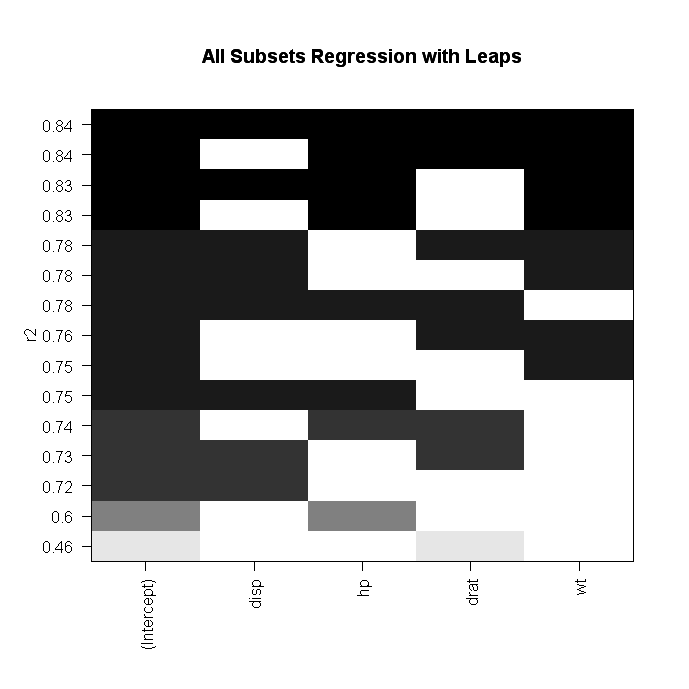
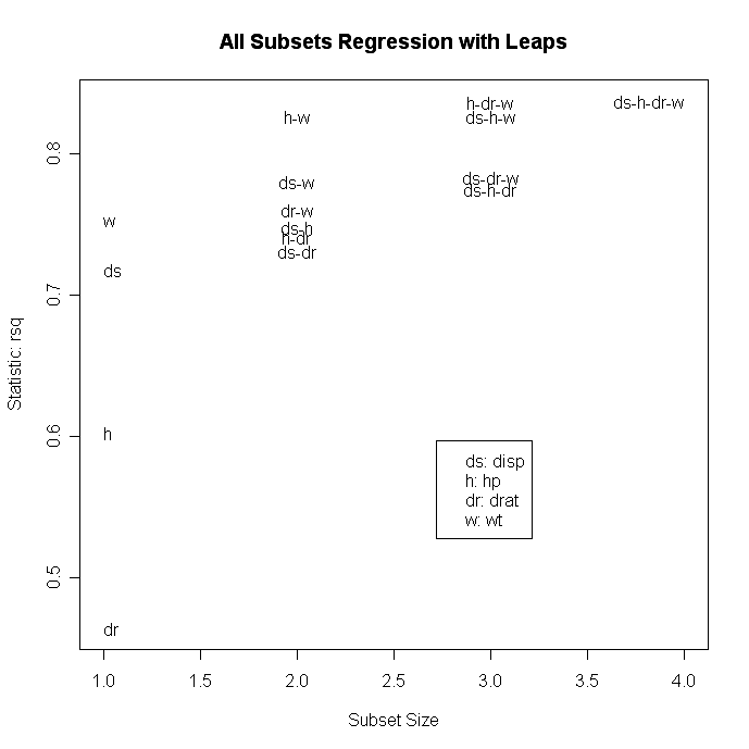
Alternatively, you can perform all-subsets regression using the leaps( ) function from the leaps package. In the following code nbest indicates the number of subsets of each size to report. Here, the ten best models will be reported for each subset size (1 predictor, 2 predictors, etc.).
# mydataをdat2に変えれば上述のデータセットに以下のコードが適用される
# All Subsets Regression

				library(leaps)

				attach(mydata)

				leaps<-regsubsets(y~x1+x2+x3+x4,data=mydata,nbest=10)

				# view results

				summary(leaps)

				# plot a table of models showing variables in each model.

				#
			models   are ordered by the selection statistic.

			plot(leaps,scale="r2")

			# plot statistic by subset size

			library(car)

			subsets(leaps, statistic="rsq")
 click to view
Other options for plot( ) are bic, Cp, and adjr2. Other options for plotting with
subset( ) are bic, cp, adjr2, and rss.
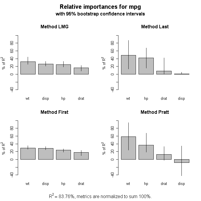
相対重要度 (Relative Importance)
これもよくわからない。わからないことがおおいものだ。The relaimpo package provides measures of relative importance for each of the predictors in the model. See help(calc.relimp) for details on the four measures of relative importance provided.
# Calculate Relative Importance for Each Predictor

					library(relaimpo)

calc.relimp(fit,type=c("lmg","last","first","pratt"),

   rela=TRUE)


				# Bootstrap Measures of Relative Importance (1000 samples)

boot <- boot.relimp(fit, b = 1000, type = c("lmg",

  "last", "first", "pratt"), rank = TRUE,

  diff = TRUE, rela = TRUE)

				booteval.relimp(boot) # print result

plot(booteval.relimp(boot,sort=TRUE)) # plot result
 click to view
グラフ化のススメ
car パッケージは 回帰診断 や 散布図を含め、いろいろなプロット法を提供している
Going Further
非線形回帰 (Nonlinear Regression)
nls パッケージには非線形回帰の関数がある。John Foxの Nonlinear Regression and Nonlinear Least Squares 参照。Huetらの書籍も有用。 Statistical Tools for Nonlinear Regression: A Practical Guide with S-PLUS and R Examples (amazon.comリンク)
ロバスト回帰 (Robust Regression) のリンク
- John Fox's Robust Regression
- UCLA Statistical Computing website: Robust Regression Examples
- robustパッケージ
- robustbaseパッケージ
- David Olive Applied Robust Statistics. Rコードつき
交互作用のある重回帰
文献
Aiken, L. S., & West, S. G. (1991). Multiple Regression: Testing and interpreting interactions . Newbury Park, CA: Sage.
Cohen, J., Cohen, P., West, S. G., & Aiken, L. S. (2003). Applied multiple regression/correlation analysis for the behavioral sciences (3rd ed.). Mahwah, NJ: Erlbaum.
		# 交互作用重回帰の別の例。以下参考。感謝

		# http://faculty.chicagobooth.edu/wilhelm.hofmann/index.html

		library(foreign)

		dat <- read.spss("http://file.scratchhit.pazru.com/c5b01bb9.sav", to.data.frame=T, max.value.labels=99)

		head(dat)


		# 記述統計

		library(psych)

		describe(dat)

		x <- dat[c(6,2,3,4)]


		attach(dat)

		idv <- height

		mod <- age

		dv <- lifesat

		idvc <- scale(idv, scale=F)

		modc <- scale(mod, scale=F)

		summary(lm(dv~idvc*modc))


		# simple slope

		modch <- modc-sd(modc)

		hmod <- lm(dv~idvc*modch)

		summary(hmod) # idvcの結果を参照する。sdの足し引きをしてないほう。

		modcl <- modc+sd(modc)

		lmod <- lm(dv~idvc*modcl)

		summary(lmod) # idvcの結果を参照する。sdの足し引きをしてないほう。

		# spssの結果。上記解説ページより、単純傾斜の結果スライドだけ抜粋


		# プロット

		# 独立変数と従属変数のxyプロットを作成し、それを調整変数がどう調整しているかを示す。

		x <- idvc

		y <- dv

		plot(x,y, col=0)

		abline(hmod, lty=1)

		abline(lmod, lty=2)

		legend("topright", legend=c("modabove", "modbelow"), lty=1:2)


		# 正しい標準化値。交互作用項を作成してから標準化するのは誤り

		hsc <- scale(idv)

		asc <- scale(mod)

		lsc <- scale(dv)

		summary(lm(lsc~hsc*asc))


		# simple slopeの標準化値

		asch <- asc-1

		hmods <- lm(lsc~hsc*asch)

		summary(hmods) # 高群

		modcl <- asc+1

		lmods <- lm(lsc~hsc*modcl)

		summary(lmods) # 低群


		# 標準化値のプロット

		win.graph()

		x <- asc

		y <- lsc

		plot(x,y, col=0)

		abline(hmods, lty=1)

		abline(lmods, lty=2)

		legend("topright", legend=c("modabove", "modbelow"), lty=1:2)


		# 連続 x カテゴリカル

		summary(lm(dv~idvc*gender))


		# simple slope

		 mm <- factor(gender, levels=c("male", "female")) # 男性をリファレンスカテゴリにする。ダミーコードではmale=0, female=1になる。

		 ff <- factor(gender, levels=c("female", "male"))

		 summary(lm(dv~idvc*mm)) # 男性

		 summary(lm(dv~idvc*ff)) # 女性


		# 標準化値

		# The unstandardized solution from the output is the correct solution (Friedrich, 1982)!

		summary(lm(lsc~hsc*gender))

		 # .507 = estimated difference in regression weights between groups

		# simple slope. カテゴリカル変数は標準化しないこと

		 summary(lm(lsc~hsc*mm)) # 男性

		 summary(lm(lsc~hsc*ff)) # 女性


		# プロット

		plot(idvc, dv)

		abline(lm(dv~idvc*mm), lty=1)

		abline(lm(dv~idvc*ff), lty=2)

		legend("bottomright", legend=c("male", "female"), lty=1:2)


		# x軸とライン分けを変えたプロット

		 lmres <- lm(dv~idvc*gender) # 全体のモデル

		 coef(lmres)

		 inc <- coef(lmres)[1] # 全体の切片

		 cfidv <- coef(lmres)[2] # 独立変数の回帰係数

		 cfmod <- coef(lmres)[3] # 調整変数の回帰係数

		 cfint <- coef(lmres)[4] # 独立変数の回帰係数

		 sdidv <- sd(idvc)


		 # 全体の重回帰分析でfemaleをリファレンスカテゴリにしている場合

		 fh <- inc+sdidv*cfidv # 切片+(平均+1SD)*回帰係数

		 fl <- inc-sdidv*cfidv # 切片+(平均-1SD)*回帰係数

		 mh <- inc+sdidv*cfidv + cfmod+((sdidv)*cfint) # 切片+(平均+1SD)*回帰係数 + 調整変数の回帰係数+((平均+1SD)*交互作用項の回帰係数)

		 ml <- inc-sdidv*cfidv + cfmod-((sdidv)*cfint) # 切片+(平均-1SD)*回帰係数 + 調整変数の回帰係数+((平均-1SD)*交互作用項の回帰係数)


		 mat <- matrix(c(fl, ml, fh, mh), nr=2, dimnames=list(c("female", "male"), c("idvlow", "idvhigh")))

		 mat

		 matplot(mat, type="l", xaxt="n")

		 axis(1,

		     at = 1:2,

		     labels=rownames(mat),

		     )

		 legend("bottomleft", legend=colnames(mat), lty=1:2, col=1:2)

		# 棒グラフにしてみる

		win.graph(); barplot(t(mat), beside=T, legend=c("idvlow", "idvhigh"), ylab="dv")
多変量重回帰分析
ヨーク大の講義ページの資料
どうもこうしたものの図示にはHEプロットというのを使うらしい。Jon Foxがつくっていた。すごい。
ヨーク大のMichael Friendlyさんが偉い人らしい。そのうち調べよう。
	library(car)

	hsb2 <- read.table('http://www.ats.ucla.edu/stat/R/faq/hsb2.csv', header=T, sep=",")

	result <- Manova(lm(cbind(write,read)~female+math+science+socst, hsb2))

	summary(result)