回帰診断
car パッケージで回帰診断が行える。
以下参考
# まずは普通に重回帰分析。データおよびSPSSの結果は右から:SPSS Web Books  Regression with SPSS  Chapter 2 - Regression Diagnostics


				library(foreign)

				dat <- read.spss("http://www.ats.ucla.edu/stat/spss/webbooks/reg/crime.sav", to.data.frame=T)

				names(dat) <- tolower(names(dat))

				head(dat)


				fit <- lm(crime~pctmetro+poverty+single, data=dat)

				summary(fit)


				library(car)
外れ値
outlierTest(fit) # Bonferonni 法でp値を調整
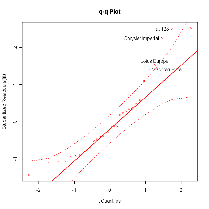
qqPlot(fit, main="QQ Plot") #qq plot スチューデント残差のqqプロット
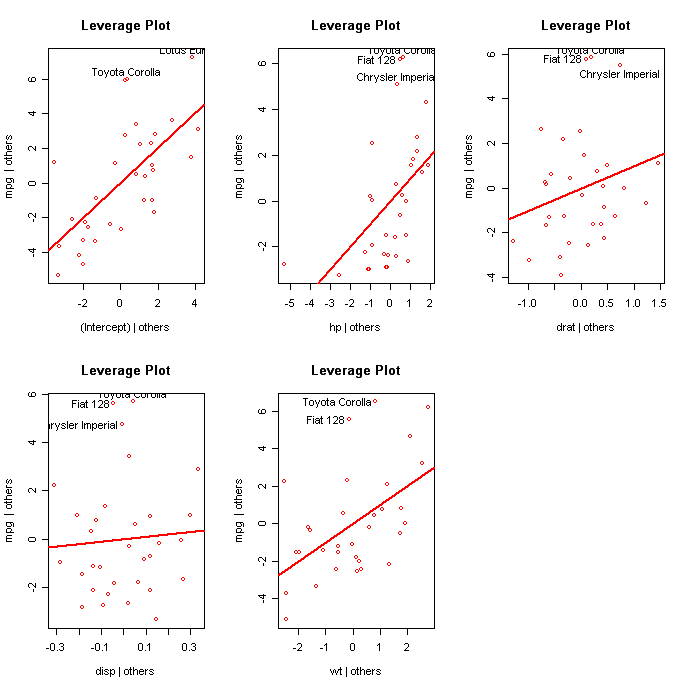
leveragePlots(fit) # レベレッジプロット
 click to view
影響の大きい観測値
# 影響の大きい観測値をプロット
avPlots(fit)
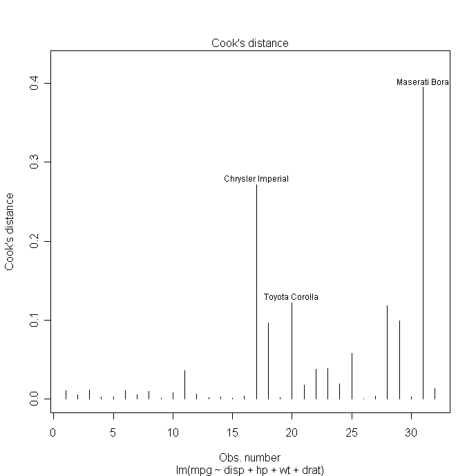
# Cook's D プロット
# D 値は > 4/(n-k-1)
cutoff <- 4/((nrow(dat)-length(fit$coefficients)-2))
plot(fit, which=4, cook.levels=cutoff)
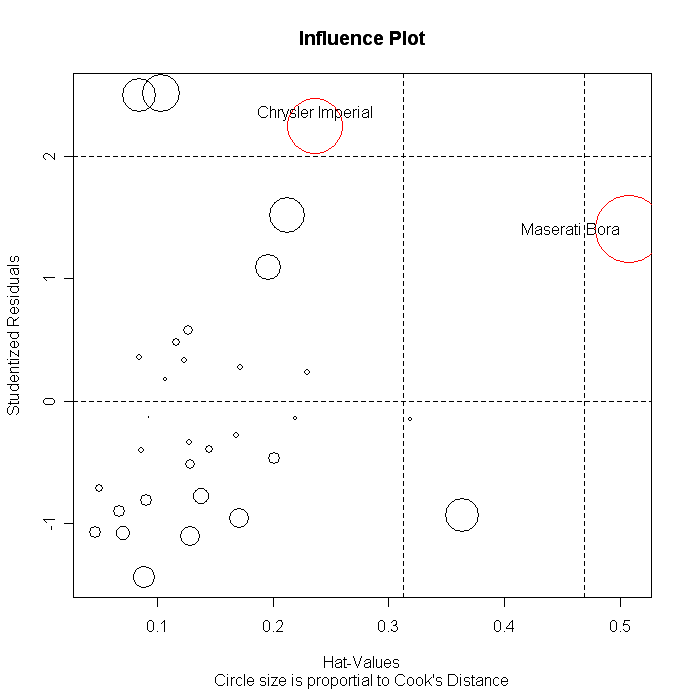
# Influence Plot
influencePlot(fit, main="Influence Plot", sub="Circle size is proportial to Cook's Distance" )

 click to view
正規性
# スチューデント化された残差のqqプロットにより残差の正規性を調べる

					 qqPlot(fit, main="QQ Plot")


					 #スチューデント化された残差の分布

					library(MASS)

					 sresid <- studres(fit)

					 hist(sresid, freq=FALSE,

					    main="Distribution of Studentized Residuals")

					 xfit<-seq(min(sresid),max(sresid),length=40)

					 yfit<-dnorm(xfit)

					 lines(xfit, yfit)


lines(xfit, yfit)
 click to view
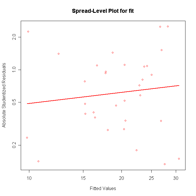
誤差分散の等質性
				# 等分散性 homoscedasticity の評価

					ncvTest(fit)


				# 残差と予測値のプロット

				spreadLevelPlot(fit)
 click to view
多重共線性 Multi-collinearity
				vif(fit) # variance inflation factors
				sqrt(vif(fit)) > 2 # problem?
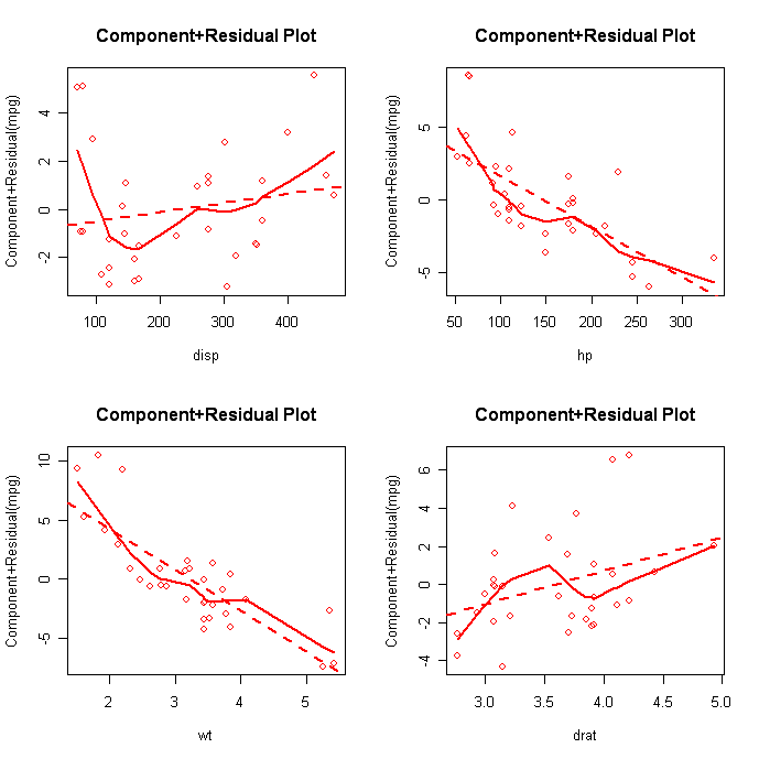
線形性 Nonlinearity
				# 要素 + 残差 plot

				 crPlots(fit)


				 # Ceres plots

				 ceresPlots(fit)
 click to view
誤差の独立性 Non-independence of Errors
				# 誤差項の系列相関に関するダービン・ワトソンの検定

				durbinWatsonTest(fit)
他のヘルプ
gvlma パッケージのgvlma( ) 関数で尖度、歪度、分散の不均一性を評価できる。.
					library(gvlma)

					gvmodel <- gvlma(fit)


					summary(gvmodel)
Going Further
もっと勉強するには以下を見よう。
Applied regression analyses, linear models, and related methods
An R and S-Plus companion to applied regression