確率プロット
講義やデモに使う確率プロット
RjpwikiのRにおける確率分布も参照。
| 分布名 | Rの名前 | 分布名 | Rの名前 |
| ベータ | beta | 対数正規 | lnorm |
| 二項 | binom | 負の2項 | nbinom |
| コーシー | cauchy | 正規 | norm |
| カイ二乗 | chisq | ポアソン | pois |
| 指数 | exp | スチューデントのt | t |
| F | f | 一様 | unif |
| ガンマ | gamma | テューキー | tukey |
| 幾何 | geom | ワイブル | weib |
| 超幾何 | hyper | ウィルコクソン | wilcox |
| ロジスティック | logis |
For a comprehensive list, see Statistical Distributions on the R wiki.
それぞれの分布には以下のフォーマットの関数が使えるThe functions available for each distribution follow this format:
| name | description |
| d分布名( ) | 確率密度関数。例: plot(dnorm, -4, 4) |
| p分布名( ) | 累積確率関数。例: pnorm(1.96) -> 0.9750021 |
| q分布名( ) | クォンタイル値を求める。例: qnorm(0.975) -> 1.959964 |
| r分布名( ) | 乱数生成 |
使い方
pnorm(0): 標準正規分布で0より左の面積の割合を求める。
qnorm(0.9): 90%の面積になるクォンタイル値
rnorm(100) : 正規分布にもとづく乱数を100個生成
使用例1
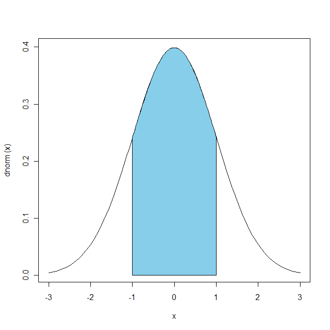
# 平均プラスマイナス1SDに約68パーセントが含まれる
pnorm(1)-pnorm(-1)
# 正規分布曲線と塗りつぶし
# 正規分布曲線
plot(dnorm, -3, 3)
# 平均プラスマイナス1SD
uv <- 1
lv <- -1
# uvとlvで指定した範囲を塗りつぶし
xvs <- seq(lv,uv,length=100) # 塗りつぶす範囲 (x軸) を指定。-1sdから+1sd
yvs <- dnorm(xvs) # 塗りつぶす範囲 (y軸) を指定
polygon(x=c(xvs, rev(xvs)), y=c(rep(0, 100), rev(yvs)), col="skyblue")
# border=0で境界線を描画しない
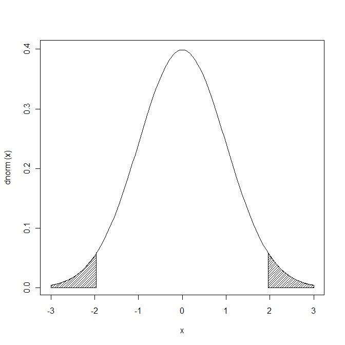
# 有意水準5%を斜線で塗りつぶし。斜線はdensity=, angle=で指定
plot(dnorm, -3, 3)
# 上側
uv <- 3; (lv <- qnorm(0.975))
xvs <- seq(lv,uv,length=100) ; yvs <- dnorm(xvs)
polygon(x=c(xvs, rev(xvs)), y=c(rep(0, 100), rev(yvs)), density=30, angle=45)
# 下側
uv <- qnorm(0.025); lv <- -3
xvs <- seq(lv,uv,length=100) ; yvs <- dnorm(xvs)
polygon(x=c(xvs, rev(xvs)), y=c(rep(0, 100), rev(yvs)), density=30, angle=45)
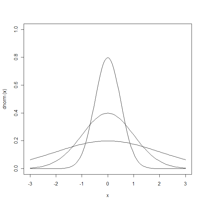
# 重ねがき。ばらついた分布とばらついてない分布
x <- seq(-3, 3, 0.01)
plot(dnorm, -3, 3, ylim=c(0,1)) # sd=1
curve(dnorm(x=x, mean=0, sd=2), type="l", add=T) # sd=2
# なんだかわからないが、"x"というオブジェクトを使わないとエラーになる
curve(dnorm(x=x, mean=0, sd=0.5), type="l", add=T) # sd=0.5
# 参考: http://cse.niaes.affrc.go.jp/minaka/R/R-normal.html
 click to view
 click to view
 click to view
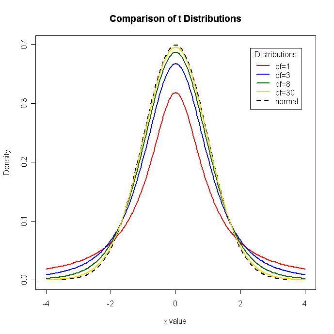
使用例2
# 色々な自由度のt分布


					x		<- seq(-4, 4, length=100)

					hx	 <- dnorm(x)


					degf   <- c(1, 3, 8, 30)

					colors <- c("red", "blue", "darkgreen", "gold", "black")

					labels <- c("df=1", "df=3", "df=8", "df=30", "normal")


					plot(x, hx, type="l", lty=2, xlab="x value",

				  ylab="Density", main="Comparison of t Distributions")


				for (i in 1:4){

				  lines(x, dt(x,degf[i]), lwd=2, col=colors[i])

				}


				legend("topright", inset=.05, title="Distributions",

				  labels, lwd=2, lty=c(1, 1, 1, 1, 2), col=colors)
 click to view
使用例3
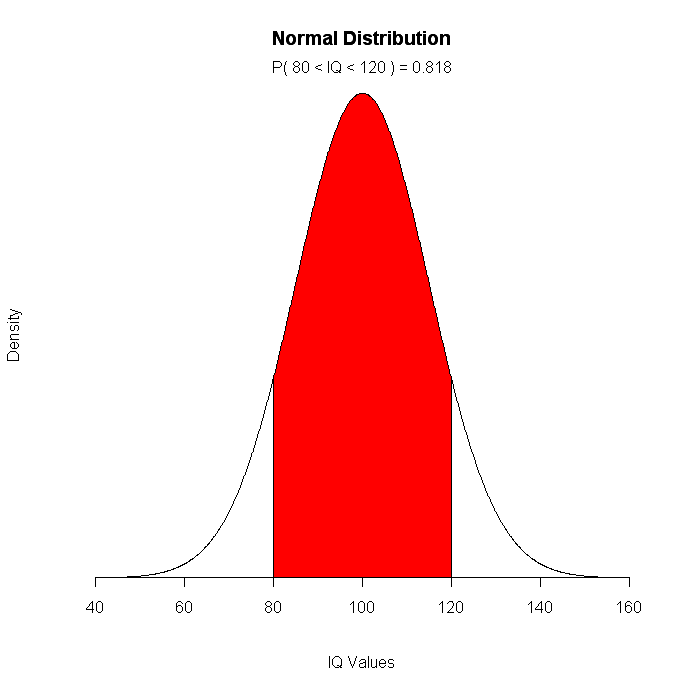
				# IQは平均100、sd15の正規分布である。80から120の人の割合は?


					mean=100; sd=15

					lb=80; ub=120


					x <- seq(-4,4,length=100)*sd + mean

					hx <- dnorm(x,mean,sd)


					plot(x, hx, type="n", xlab="IQ Values", ylab="Density",

					  main="Normal Distribution", axes=FALSE)


					i <- x >= lb & x <= ub

					lines(x, hx)

					polygon(c(lb,x[i],ub), c(0,hx[i],0), col="red")


					area <- pnorm(ub, mean, sd) - pnorm(lb, mean, sd)

					result <- paste("P(",lb,"< IQ <",ub,") =",

					   signif(area, digits=3))

					mtext(result,2)
 click to view
参考: Vincent Zonekynd's Probability Distributions.
分布への適合
qqnorm( ) 関数はQ-Qプロットをつくって正規分布へのあてはまりを評価できる。正規分布以外の理論分布でも使用可能。
				par(mfrow=c(1,2))


				# サンプルデータの生成

				x <- rt(100, df=3)


				# 正規分布への適合

					qqnorm(x);
					qqline(x)


					# 自由3のt分布への適合

					qqplot(rt(1000,df=3), x, main="t(3) Q-Q Plot",

  				ylab="Sample Quantiles")

				abline(0,1)
 click to view
MASS パッケージのfitdistr( ) 関数は単変量分布に対する最尤推定の適合を評価できる。フォーマットはfitdistr(x, densityfunction) 。xにはデータ、densityfunctionは以下のいずれかを指定 ( "beta", "cauchy", "chi-squared", "exponential", "f", "gamma", "geometric", "log-normal", "lognormal", "logistic", "negative binomial", "normal", "Poisson", "t" or "weibull")
# 対数正規分布を仮定したパラメータ推定


				# データ生成

					x <- rlnorm(100)


					# パラメータ推定

					library(MASS)

					fitdistr(x, "lognormal")
Rはカイ二乗、コルモゴロフ-スミルノフ、アンダーソン-ダーリング等、様々な分布への適合を検定できる。詳しくは Vito Ricci's Fitting Distributions with R や、Bill Huber's Fitting Distributions to Data を参照。