クラスター分析
R では様々なクラスター分析を行うことができる (cran task view)。本稿では階層的凝集法 (hierarchical agglomerative) 、分割法 (partitioning) 、モデルベース法 (model based) について説明する。絶対に正しいという手法はないので注意。
参考
データの準備
欠損値を省いておくこと。
				# 足立浩平 (2006). 多変量データ解析法――心理・教育・社会系のための入門―― ナカニシヤ出版の第2章から。感謝

				mat <- matrix(c(3.2, 3.4, 3, 3.2, 4.2, 4, 4, 3.7, 3.6, 3.6, 3.7, 3.4, 3.2, 3.2, 2.7, 3.5, 3.2, 3.2, 4.6, 4, 4.8, 4.6, 4.3, 3.6, 3.2, 3.7, 3.2, 3.8, 3.7, 3.4, 3.5, 3.5, 4.5, 3.8, 3.9, 4.1, 3.7, 3.5, 3.7, 3.5, 3.6, 3.8, 2.8, 2.5, 2.2, 2.6, 3.1, 3.4, 3.5, 3.4, 2.9, 3.5, 3.9, 3.1, 2.9, 2.8, 2.6, 2.2, 2.1, 2.5, 3, 3.2, 3.8, 4, 3.5, 4.2, 4.7, 2.7, 2.2, 2.3, 2.6, 2.6, 2.2, 2.6, 3.2, 3.1, 3.7, 4.1, 3.6, 4.2, 4.7, 2.4, 2.5, 2.4, 2.2, 3.2, 3.3, 3.6, 2.8, 2.4, 3.2, 4.3, 4.7, 3.5, 4.9, 2.3, 3.3, 3.9, 1.4, 2.1, 3.4, 2.9, 3.3, 1.5, 2.1, 3.4, 4.2, 3.5, 3.5, 1.8, 3.3, 2.5, 1.7, 3.6, 4.1, 4.2, 4.1, 1.6, 2.6, 3.5, 4.1, 3.7, 4.2, 2.3, 3.4, 4.7, 3.3, 4.1, 3.4, 3.2, 4.5, 3.7, 3.7, 4.2, 3.9, 3.5, 3.7, 3.3, 2.8, 3.9, 3.8, 4.7, 1.3, 1.5, 2.3, 3.9, 3.6, 4.4, 3.7, 2.5, 2.8, 2.9, 1.8, 2.3, 1.8, 4.2, 4.3, 4, 4.9, 3, 4.5, 4, 5, 3.5, 4.1, 3.3, 4.3, 4.3),

				nr=14,

				dimnames=list(c("僧侶", "銀行員", "漫画家", "デザイナー", "保母", "大学教授", "医師", "警察官", "新聞記者", "船乗り", "プロスポーツ選手", "作家", "俳優", "スチュワーデス"),

				c("立派な", "役立つ", "よい", "大きい", "力がある", "強い", "速い", "騒がしい", "若い", "誠実な", "かたい", "忙しい"))

				)


				smat <- scale(mat) # 標準化
分割法
K平均法 (K-means) は最もポピュラーな分割法である。この手法は事前にいくつのクラスターを抽出するか決めておく必要がある。クラスターの数で平方和をプロットしてみると、参考になるだろう。因子分析でいうスクリープロットのようなものである。 Everitt & Hothorn (pg. 251) も参考。
				# クラスターの数を決める

				wss <- (nrow(smat)-1)*sum(apply(smat,2,var))

				for (i in 2:12) wss[i] <- sum(kmeans(smat, centers=i)$withinss)

				# プロット

				plot(1:12, wss, type="b", xlab="Number of Clusters", ylab="Within groups sum of squares")


				# K平均クラスタリング

				fit <- kmeans(smat, 3) # 3 cluster solution

				# クラスターの平均

				aggregate(smat,by=list(fit$cluster),FUN=mean)

				# クラスターの割り当て (表2.3)

				data.frame(fit$cluster)
K-means関数のほかに、fpc パッケージのpam, pamk関数を使うこともできる。
階層的凝集法
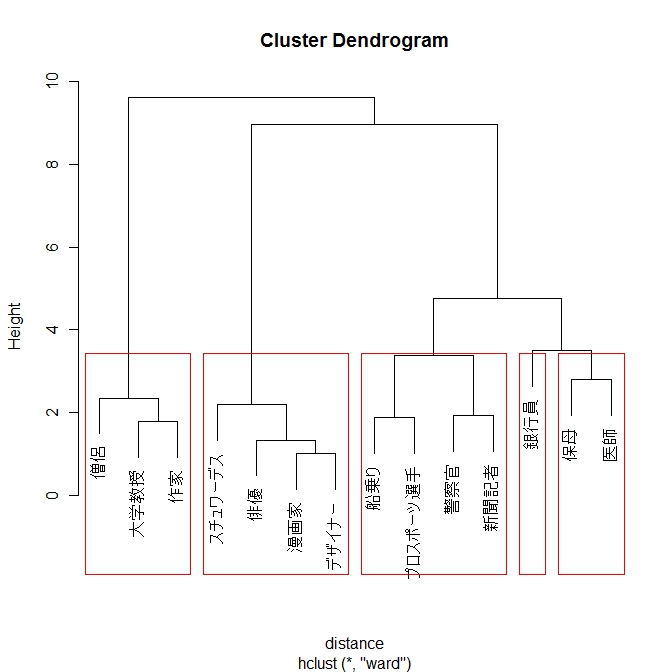
階層的クラスター分析の手法はいろいろある。以下ではウォード法について記す。
				distance <- dist(mat, method="euclidean") # ユークリッド距離の行列。教科書に従い、標準化しないデータを用いる

				fit <- hclust(distance, method="ward")

				plot(fit)


				groups <- cutree(fit, k=5) # 5クラスターに分けた場合

				data.frame(groups)

				rect.hclust(fit, k=5, border="red")  # デンドログラムで5クラスターを表現
 click to view
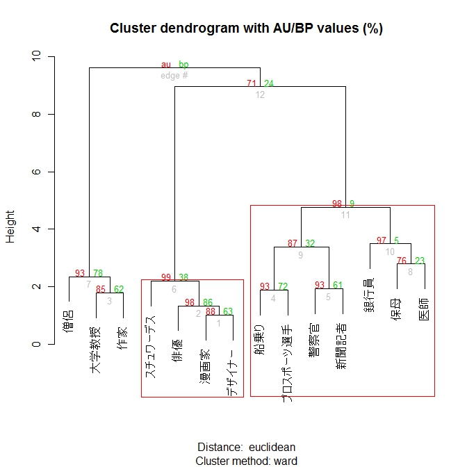
pvclustパッケージのpvclust( )関数を使うと、マルチスケール・ブートストラップ法によるp値がわかる。詳しくは作者である下平先生のページ参照。
# ウォード法とブートストラップによるp値

				library(pvclust)

				fit <- pvclust(t(mat), method.hclust="ward", method.dist="euclidean")

				plot(fit)

				# 有意なグループをハイライト

				pvrect(fit, alpha=.95)
 click to view
モデルベース法
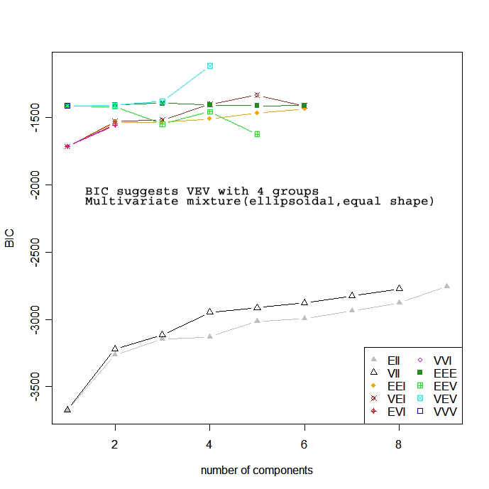
モデルベースのクラスター分析は様々なモデルを仮定し、最尤法やベイズ基準、クラスターの数でモデルの適合度を検討する。mclustパッケージのMclust( ) 関数は混合正規分布 (gaussian mixture model) に従う階層的クラスタリングで初期化したEMのBICに従い最適なモデルを求める (なんのこっちゃ) 。
					library(mclust)
					fit <- Mclust(mat)
					plot(fit, mat)
					print(mat)
 click to view
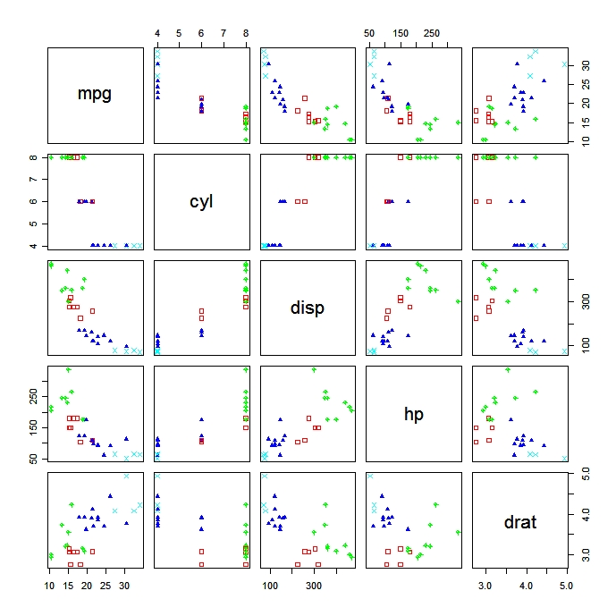
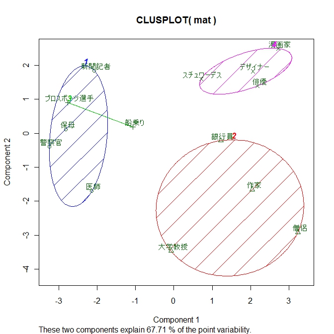
クラスター分析の結果をプロットする
# K平均法でクラスター分析

					fit <- kmeans(mat, 4)


					# 第1、第2主成分でプロット。足立 (2006) p20 図2.9 (A)

					library(cluster)


					clusplot(mat, fit$cluster, color=TRUE, shade=TRUE, labels=2, lines=0)


					# 第1、第2判別関数でプロット

					library(fpc)

					plotcluster(mydata, fit$cluster)
 click to view
クラスター解の妥当性
fpcパッケージのcluster.stats() 関数は2つのクラスター解を比較できる。基準にはHubert's gamma coefficient, the Dunn index and the corrected rand indexなどさまざま。
				library(fpc)

					cluster.stats(d, fit1$cluster, fit2$cluster)
dが距離行列の場合、fit1$cluster 、 fit$clusteは同じデータに対する2つのクラスター分析の結果を含む。