Tree-Based Models
Recursive partitioning is a fundamental tool in data mining. It helps us explore the stucture of a set of data, while developing easy to visualize decision rules for predicting a categorical (classification tree) or continuous (regression tree) outcome. This section briefly describes CART modeling, conditional inference trees, and random forests.
CART Modeling via rpart
Classification and regression trees (as described by Brieman, Freidman, Olshen, and Stone) can be generated through the rpart package. Detailed information on rpart is available in An Introduction to Recursive Partitioning Using the RPART Routines. The general steps are provided below followed by two examples.
1. Grow the Tree
To grow a tree, use
rpart(formula, data=, method=,control=) where
| formula | is in the format outcome ~ predictor1+predictor2+predictor3+ect. |
| data= | specifies the dataframe |
| method= | "class" for a classification tree "anova" for a regression tree |
| control= | optional parameters for controlling tree growth. For example, control=rpart.control(minsplit=30, cp=0.001) requires that the minimum number of observations in a node be 30 before attempting a split and that a split must decrease the overall lack of fit by a factor of 0.001 (cost complexity factor) before being attempted. |
2. Examine the results
The following functions help us to examine the results.
| printcp(fit) | display cp table |
| plotcp(fit) | plot cross-validation results |
| rsq.rpart(fit) | plot approximate R-squared and relative error for different splits (2 plots). labels are only appropriate for the "anova" method. |
| print(fit) | print results |
| summary(fit) | detailed results including surrogate splits |
| plot(fit) | plot decision tree |
| text(fit) | label the decision tree plot |
| post(fit, file=) | create postscript plot of decision tree |
In trees created by rpart( ), move to the LEFT branch when the stated condition is true (see the graphs below).
3. prune tree
Prune back the tree to avoid overfitting the data. Typically, you will want to select a tree size that minimizes the cross-validated error, the xerror column printed by printcp( ).
Prune the tree to the desired size using
prune(fit, cp= )
Specifically, use printcp( ) to examine the cross-validated error results, select the complexity parameter associated with minimum error, and place it into the prune( ) function. Alternatively, you can use the code fragment
fit$cptable[which.min(fit$cptable[,"xerror"]),"CP"]
to automatically select the complexity parameter associated with the smallest cross-validated error. Thanks to HSAUR for this idea.
Classification Tree example
Let's use the dataframe kyphosis to predict a type of deformation (kyphosis) after surgery, from age in months (Age), number of vertebrae involved (Number), and the highest vertebrae operated on (Start). # Classification Tree with rpart
library(rpart)
# grow tree
fit <- rpart(Kyphosis ~ Age + Number + Start,
method="class", data=kyphosis)
printcp(fit) # display the results
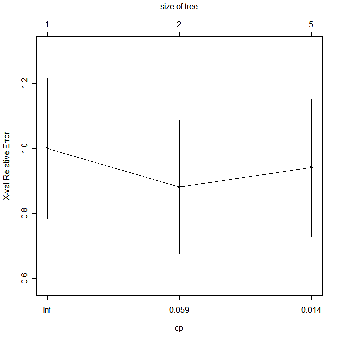
plotcp(fit) # visualize cross-validation results
summary(fit) # detailed summary of splits
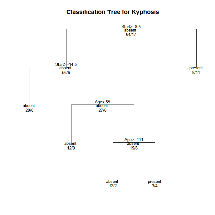
# plot tree
plot(fit, uniform=TRUE,
main="Classification Tree for Kyphosis")
text(fit, use.n=TRUE, all=TRUE, cex=.8)
# create attractive postscript plot of tree
post(fit, file = "c:/tree.ps",
title = "Classification Tree for Kyphosis")
 click to view
					# prune the tree

					pfit<- prune(fit, cp=   fit$cptable[which.min(fit$cptable[,"xerror"]),"CP"])


					# plot the pruned tree

					plot(pfit, uniform=TRUE,

  				main="Pruned Classification Tree for Kyphosis")

					text(pfit, use.n=TRUE, all=TRUE, cex=.8)

			post(pfit, file = "c:/ptree.ps",

  				title = "Pruned Classification Tree for Kyphosis")

 click to view
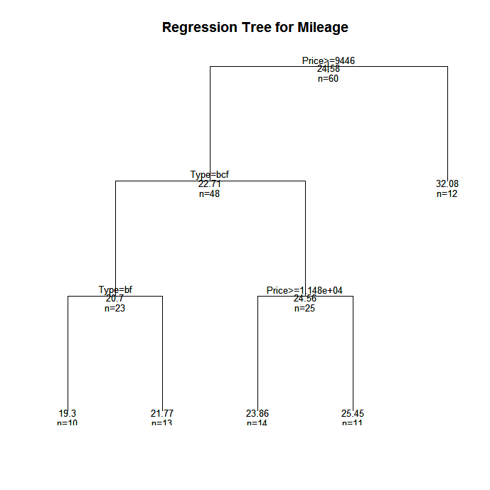
Regression Tree example
In this example we will predict car mileage from price, country, reliability, and car type. The dataframe is cu.summary.
# Regression Tree Example
library(rpart)
# grow tree
fit <- rpart(Mileage~Price + Country + Reliability + Type,
method="anova", data=cu.summary)
printcp(fit) # display the results
plotcp(fit) # visualize cross-validation results
summary(fit) # detailed summary of splits
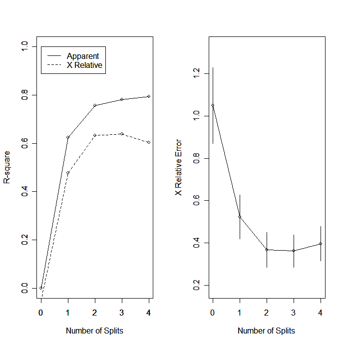
# create additional plots
par(mfrow=c(1,2)) # two plots on one page
rsq.rpart(fit) # visualize cross-validation results
# plot tree
plot(fit, uniform=TRUE,
main="Regression Tree for Mileage ")
text(fit, use.n=TRUE, all=TRUE, cex=.8)
# create attractive postcript plot of tree
post(fit, file = "c:/tree2.ps",
title = "Regression Tree for Mileage ")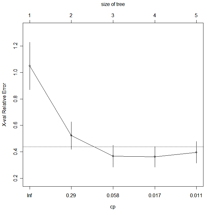
 click to view
# prune the tree

pfit<- prune(fit, cp=0.01160389) # from cptable


# plot the pruned tree

plot(pfit, uniform=TRUE,

  				main="Pruned Regression Tree for Mileage")

text(pfit, use.n=TRUE, all=TRUE, cex=.8)

post(pfit, file = "c:/ptree2.ps",

  				title = "Pruned Regression Tree for Mileage")
It turns out that this produces the same tree as the original.
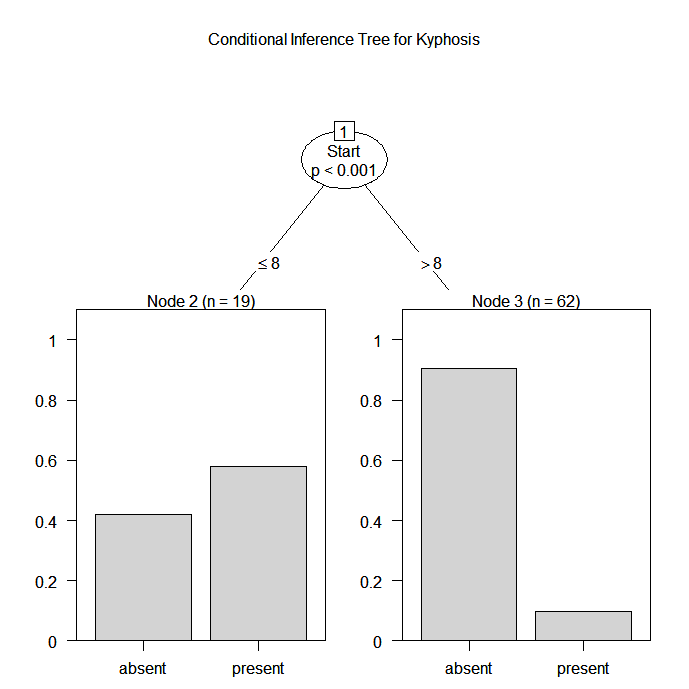
conditional inference trees via party
The party package provides nonparametric regression trees for nominal, ordinal, numeric, censored, and multivariate responses. party: A laboratory for recursive partitioning, provides details.
You can create a regression or classification tree via the function
ctree(formula, data=)
The type of tree created will depend on the outcome variable (nominal factor, ordered factor, numeric, etc.). Tree growth is based on statistical stopping rules, so pruning should not be required.
The previous two examples are re-analyzed below.
# Conditional Inference Tree for Kyphosis

library(party)

fit <- ctree(Kyphosis ~ Age + Number + Start,

   data=kyphosis)

plot(fit, main="Conditional Inference Tree for Kyphosis")
 click to view
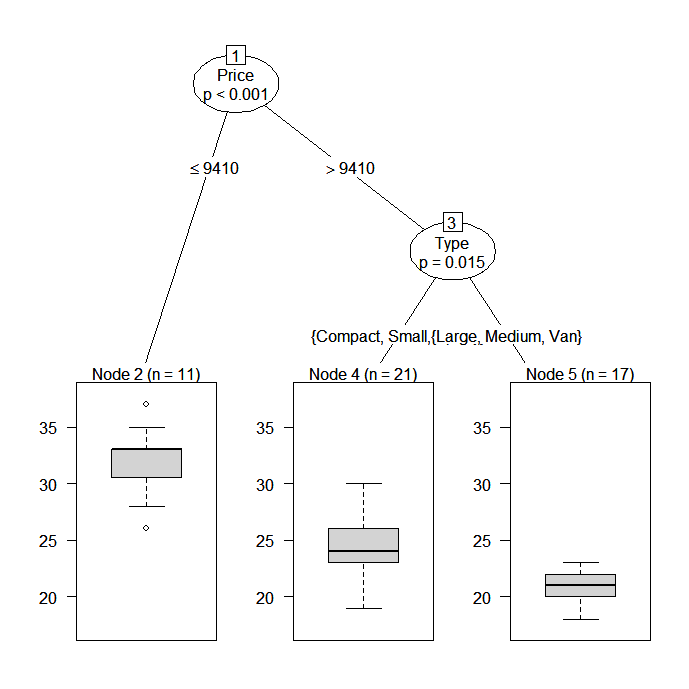
# Conditional Inference Tree for Mileage

					library(party)

fit2 <- ctree(Mileage~Price + Country + Reliability + Type,

   data=na.omit(cu.summary))
 click to view
Random Forests
Random forests improve predictive accuracy by generating a large number of bootstrapped trees (based on random samples of variables), classifying a case using each tree in this new "forest", and deciding a final predicted outcome by combining the results across all of the trees (an average in regression, a majority vote in classification). Breiman and Cutler's random forest approach is implimented via the randomForest package.
Here is an example.
# Random Forest prediction of Kyphosis data

					library(randomForest)

					fit <- randomForest(Kyphosis ~ Age + Number + Start,   data=kyphosis)

					print(fit) # view results


				importance(fit) # importance of each predictor
For more details see the comprehensive Random Forest website.
Going Further
This section has only touched on the options available. To learn more, see the CRAN Task View on Machine & Statistical Learning.